Univariate anomaly detection

This part of the pipeline detects anomalies on a single time series. It consists of a training part (baseline creation) that periodically (every 24 hours) determines the normal behaviour of the time series and a detection (live anomaly detection) part that close to real-time determines if behaviour is different from the one observed in the past (an anomaly) is ongoing is.

Baseline creation

Data selection

Among all the data available, we select those that are useful to describe the current situation: we give the highest weight to the most recent data and those containing recursive behaviour (daily, weekly, monthly).

There are often cycles and seasonal behavior in the data; therefore, historical data have a higher weight when baselining. For example, in many cases, the behaviour 24 hours ago is more representative of the situation now than the behaviour 13 hours ago (daily cycle). Or the behaviour one week ago is more significant than the one 5 weeks ago. The current version uses a static selection, the same for all the time series, with the same weight. This is very lightweight as we don’t have to learn the weights for each metric, making this model easily scalable. Common sense is used for this selection: recent data matter more, and we use daily, weekly, and monthly cycles. This makes the model equivalent to a hybrid between clustering and a static ARIMA.

Clustering for baseline creation

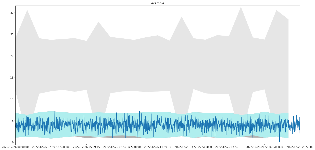
This is the part that groups the data observed in the past into different observed behaviours. the historical data are grouped into up to three different clusters. One describing the most frequent behaviour and up to two secondary behaviors, which include less frequent behaviours or past anomalies. Therefore, the approach we use is a multi-baseline behaviour, in which one baseline corresponds to the main behaviour, and the rest describe secondary behaviours which cannot be guaranteed to be anomaly free. To do this, we use univariate unsupervised clustering methods.

Creation of the baselines

The baselines that are going to be used in the anomaly detection are created. We use different models for the three different groups of time series classified in the pre-processing step.

High-Frequency High Activity

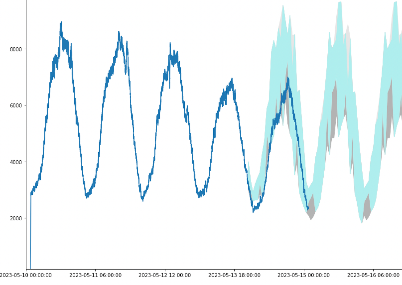
These are the metrics that are richer in information so we can make a more complete analysis. Before forming the corridor, the data are re-aggregated, considering the frequency, to treat missing data. In the case in which the data are aggregated as total, the analysis is considering the data smoothened by re-aggregating by 5 minutes, and this is to reabsorb oscillations and distinguish the case in which one metric is consistently zero for a long time from the one in which there is occasional oscillation to zero. One baseline to describe the most frequent behaviour is always formed; secondary baselines are created if enough data do not fit the main behaviour. This is done by fitting the historical data per hour and considering 3 standard deviations. Also, an autoregressive model is learned to predict the next data point based on the last data point which came in. This autoregressive model is used in the anomaly detection phase to confirm that the trend of data points diverging from the main behaviour is to be considered anomalous.

High-Frequency Low Activity Low Frequency

In the case in which the data are aggregated as total, the analysis is considering the data smoothened by re-aggregating by 5 minutes, and this is to reabsorb oscillations and distinguish the case in which one metric is consistently zero for a long time from the one in which there is occasional oscillation to zero. A single baseline describing the most frequent behaviour is formed. No autoregressive model is considered. This is because this has way less structure than the HFHA one.

Low Frequency

The data are aggregated hourly, and this is because this type of metric has only hourly anomaly detection enabled. A single baseline describing the most frequent behaviour is formed. No autoregressive model is considered.

For all three considered cases (HFHA, HFLA, LF), the details of the algorithms vary a bit according to the metric aggregation (average, total, or maximum).

Live anomaly detection

The anomaly detection works by re-aggregating the data that come in in a certain span of time. The HFHA and the HFLA anomaly detection update every minute, and the LF every hour. For each aggregated data point, we evaluate if an anomaly is ongoing. Single point anomalies are then built to a unique anomaly for anomalous points close in time: we deliver an anomaly detection that gives information on how a situation develops in time.

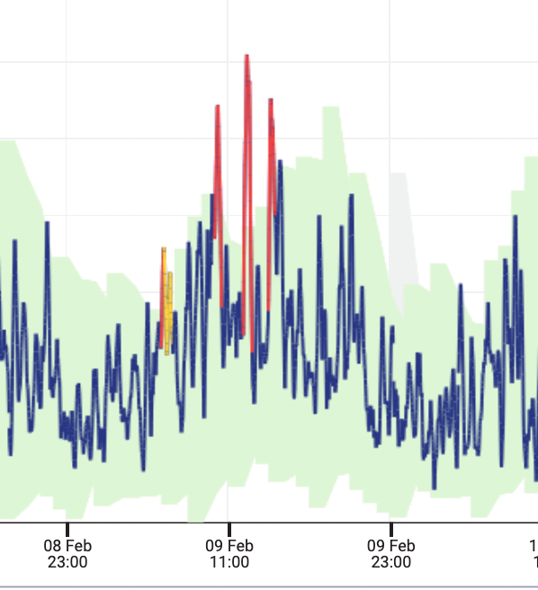
Criticality of the anomaly

For each aggregated data point, a different weight is assigned if the point is in the main baseline (in the case of HFHA can also be outside but diverge at a reasonable trend and not too far, judged by using the autoregressive model), in a secondary baseline or outside all the baselines. An anomaly score is built incrementally by averaging among these weights in time for as long as the data points are mostly outside the main baseline. This results in a measurement (the score) that, even if not rigorous, gives an “at a glance” description of the anomaly and can be averaged across nodes and systems. The score is then summarised into levels of criticality, classifying the data points into red (high probability of anomaly), orange (medium-high probability of anomaly), and yellow (medium-low probability of anomaly). A yellow anomaly has a lower likelihood of being a real anomaly than a red could also correspond to anomalies escalating or resolving. If we focus on the anomalies that are classified as red, they include the most severe deviations from behaviour seen in the past, even if they will not include all the anomalies.